If there is one prayer that you should pray/sing every day and every hour, it is the
LORD's prayer (Our FATHER in Heaven prayer)
- Samuel Dominic Chukwuemeka
It is the most powerful prayer.
A pure heart, a clean mind, and a clear conscience is necessary for it.
For in GOD we live, and move, and have our being.
- Acts 17:28
The Joy of a Teacher is the Success of his Students.
- Samuel Dominic Chukwuemeka
Differential Calculus

I greet you this day,
First: read the notes.
Second: view the videos.
Third: solve the solved examples and word problems
Fourth: check your solutions with my thoroughly-explained solutions.
Fifth: check your answers with the calculators as applicable.
Comments, ideas, areas of improvement, questions, and constructive criticisms are welcome.
If you are my student, please do not contact me here. Contact me via the school's system. Thank you for visiting.
Samuel Dominic Chukwuemeka (Samdom For Peace) B.Eng., A.A.T, M.Ed., M.S
Objectives
Students will:
(1.) Discuss the concept of the derivative of a function.
(2.) Determine the derivative of an explicit function by limit.
(3.) Determine the derivative of an explicit function by rules.
(4.) Determine the higher-order derivatives of explicit functions.
(5.) Differentiate implicit functions.
(6.) Differentiate exponential functions.
(7.) Differentiate logarithmic functions.
(8.) Differentiate trigonometric functions.
(9.) Discuss Newton's method.
(10.) Solve applied problems involving the derivatives of functions.
(11.) Solve some topics in Differential Calculus using technologies such as Wolfram|Alpha widgets and TI-84 Plus among others.
Derivatives by Limits
Derivative by Limit is the same as Derivative by Definition.
It is also known as the Derivative of a Function from First Principles.
Recall: The Difference Quotient (DQ) of a Function
The limit of the difference quotient of a function as the change in the input approaches zero is known as the derivative of the function.
Given the:
$
function: y = f(x) \\[3ex]
x = input \\[3ex]
y = f(x) = output \\[3ex]
x_1 = initial\;\;value\;\;of\;\;the\;\;input \\[3ex]
x_2 = final\;\;value\;\;of\;\;the\;\;input \\[3ex]
y_1 = initial\;\;value\;\;of\;\;the\;\;output \\[3ex]
y_2 = final\;\;value\;\;of\;\;the\;\;output \\[3ex]
h = \Delta x = x_2 - x_1 = change\;\;in\;\;the\;\;input \\[3ex]
\Delta y = y_2 - y_1 = change\;\;in\;\;the\;\;output \\[3ex]
y_2 = f(x_2) \\[3ex]
y_1 = f(x_1) \\[3ex]
slope\;\;of\;\;secant\;\;line = DQ = Difference\;\;Quotient = \dfrac{\Delta y}{\Delta x} \\[5ex]
= \dfrac{y_2 - y_1}{x_2 - x_1} \\[5ex]
= \dfrac{f(x_2) - f(x_1)}{h} \\[5ex]
Let: x_1 = x \\[3ex]
h = x_2 - x \\[3ex]
x_2 = h + x \\[3ex]
x_2 = x + h \\[3ex]
f(x_2) = f(x + h) \\[3ex]
f(x_1) = f(x) \\[3ex]
\implies \\[3ex]
DQ = \dfrac{f(x + h) - f(x)}{h} \\[5ex]
f'(x) = slope\;\;of\;\;tangent\;\;line = Derivative = \displaystyle{\lim_{h \to 0}}\: DQ \\[5ex]
f'(x) = \displaystyle{\lim_{h \to 0}}\: \dfrac{f(x + h) - f(x)}{h} \\[5ex]
$
Given: a function: say $y = f(x)$
To determine the derivative of a function by limits:
(1.) Find: $f(x + h)$
(2.) Perform: $f(x + h) - f(x)$. This is the numerator.
(3.) Simplify: as applicable.
(4.) Divide: by the denominator, $h$
(5.) Simplify as applicable.
(6.) Evaluate: the limit of the division as $h$ approaches zero.
The result is the derivative of the function.
Let us do an example.
Example 1: Determine the derivative of $y = x^2$ from first principles.
$
y' = \displaystyle{\lim_{h \to 0}}\: \dfrac{f(x + h) - f(x)}{h} \\[5ex]
y = f(x) = x^2 \\[3ex]
f(x + h) = (x + h)^2 \\[3ex]
= (x + h)(x + h) \\[3ex]
= x^2 + hx + hx + h^2 \\[3ex]
= x^2 + 2xh + h^2 \\[3ex]
\underline{Numerator} \\[3ex]
f(x + h) - f(x) \\[3ex]
= x^2 + 2xh + h^2 - x^2 \\[3ex]
= 2xh + h^2 \\[3ex]
= h(2x + h) \\[3ex]
\dfrac{Numerator}{Denominator} \\[5ex]
= \dfrac{h(2x + h)}{h} \\[5ex]
= 2x + h \\[3ex]
y' = \displaystyle{\lim_{h \to 0}}\: 2x + h \\[3ex]
y' = 2x + 0 \\[3ex]
y' = 2x
$
Derivatives by Rules
Power Rule
Pre-requisite Topic: Exponents
The Power Rule of Derivatives states that:
$
If\:\: y = x^n \\[3ex]
then\:\: \dfrac{dy}{dx} = nx^{n - 1} \\[5ex]
If\:\: y = ax^n \\[3ex]
then\:\: \dfrac{dy}{dx} = nax^{n - 1}
$
Sum/Difference Rule
The Sum Rule of Derivatives states that:
$
If\:\: y = u + v \\[3ex]
where\:\: u = f(x);\:\: v = f(x) \\[3ex]
then\:\: \dfrac{dy}{dx} = \dfrac{du}{dx} + \dfrac{dv}{dx} \\[5ex]
If\:\: y = u + v + w \\[3ex]
where\:\: u = f(x);\:\: v = f(x);\:\: w = f(x) \\[3ex]
then\:\: \dfrac{dy}{dx} = \dfrac{du}{dx} + \dfrac{dv}{dx} + \dfrac{dw}{dx}
$
The Difference Rule of Derivatives states that:
$
If\:\: y = u - v \\[3ex]
where\:\: u = f(x);\:\: v = f(x) \\[3ex]
then\:\: \dfrac{dy}{dx} = \dfrac{du}{dx} - \dfrac{dv}{dx} \\[5ex]
If\:\: y = u - v - w \\[3ex]
where\:\: u = f(x);\:\: v = f(x);\:\: w = f(x) \\[3ex]
then\:\: \dfrac{dy}{dx} = \dfrac{du}{dx} - \dfrac{dv}{dx} - \dfrac{dw}{dx}
$
You can write it in a compact form
The Sum/Difference Rule of Derivatives states that:
$
If\:\: y = u \pm v \\[3ex]
where\:\: u = f(x);\:\: v = f(x) \\[3ex]
then\:\: \dfrac{dy}{dx} = \dfrac{du}{dx} \pm \dfrac{dv}{dx} \\[5ex]
If\:\: y = u \pm v \pm w \\[3ex]
where\:\: u = f(x);\:\: v = f(x);\:\: w = f(x) \\[3ex]
then\:\: \dfrac{dy}{dx} = \dfrac{du}{dx} \pm \dfrac{dv}{dx} \pm \dfrac{dw}{dx}
$
Chain Rule
The Chain Rule is also known as the Function of a Function Rule
We shall see the reasons.
Let us begin with the reason why it is called the Function of a Function Rule
$y$ is not a direct function of $x$
Rather, it is a function of some other function that is a function of $x$
The Function of a Function Rule of Derivatives states that:
$
If\:\: y = f(u) \\[3ex]
and\:\: u = f(x) \\[3ex]
then\:\: \dfrac{dy}{dx} = \dfrac{dy}{du} * \dfrac{du}{dx} \\[5ex]
$
As you can see, $y$ is a function of $u$ which is then a function of $x$
So, $y$ is a function of a function of $x$
Student: Does this apply only to the case of three variables - $y, u, x$
where $y$ is a function of $u$ which is a function of $x$
Teacher: Good question.
No, it does not apply to only three variables.
It can apply to so many variables - sort of like a chain
Hence, the name "Chain Rule"
The Chain Rule of Derivatives states that:
$
If\:\: y = f(u) \\[3ex]
and\:\: u = f(v) \\[3ex]
and\:\: v = f(x) \\[3ex]
then\:\: \dfrac{dy}{dx} = \dfrac{dy}{du} * \dfrac{du}{dv} * \dfrac{dv}{dx} \\[5ex]
$
As you can see, this is a case of $3$ chains
$
If\:\: y = f(u) \\[3ex]
and\:\: u = f(v) \\[3ex]
and\:\: v = f(w) \\[3ex]
and\:\: w = f(x) \\[3ex]
then\:\: \dfrac{dy}{dx} = \dfrac{dy}{du} * \dfrac{du}{dv} * \dfrac{dv}{dw} * \dfrac{dw}{dx} \\[5ex]
$
This is a case of $4$ chains
Student: How do we set up the chains?
How do we know we set it up correctly?
How do we know when to use it?
Teacher: Good question.
When you see composite functions or functions with several exponents or functions that are not
"direct" sums, differences, product, or quotient; then the Chain Rule is probably the likely
rule to use
You do want to break it up into several functions as simply as possible
After setting it up and multiplying the functions, it will result to $\dfrac{dy}{dx}$
All the terms will cancel out leaving only the $\dfrac{dy}{dx}$
That way, you know you set it up correctly.
If you review the $2$ chains, $3$ chains, and $4$ chains, you will notice that only the
$\dfrac{dy}{dx}$ remains.
Product Rule
The Product Rule of Derivatives states that:
$
If\:\: y = u * v \\[3ex]
where\:\: u = f(x);\:\: v = f(x) \\[3ex]
then\:\: \dfrac{dy}{dx} = u\dfrac{dv}{dx} + v\dfrac{du}{dx} \\[5ex]
$
NOTE: Before using the Product Rule, you must first express the function as the product of
only two functions.
In other words, it must be the product of only two functions.
Mnemonic to Remember Product Rule
Let:
$
y = u * v \\[3ex]
u = first \\[3ex]
v = second \\[3ex]
y = first * second \\[3ex]
\color{purple}{\dfrac{dy}{dx} = first * dee-second + second * dee-first}
$
Quotient Rule
The Quotient Rule of Derivatives states that:
$
If\:\: y = \dfrac{u}{v} \\[5ex]
where\:\: u = f(x);\:\: v = f(x) \\[3ex]
then\:\: \dfrac{dy}{dx} = \dfrac{v\dfrac{du}{dx} - u\dfrac{dv}{dx}}{v^2} \\[5ex]
$
NOTE: Before using the Quotient Rule, you must first express the function as the quotient of
only two functions.
In other words, it must be the quotient of only two functions.
Mnemonic to Remember Quotient Rule
Let:
$
y = \dfrac{u}{v} \\[5ex]
u = top \\[3ex]
v = bottom \\[3ex]
y = \dfrac{top}{bottom} \\[5ex]
\color{purple}{\dfrac{dy}{dx} = [(bottom * dee-top) \:\:minus\:\: (top * dee-bottom)] \:\:all\:\:over\:\: bottom-squared}
$
Derivatives of Basic Functions
Derivatives of Basic Trigonometric Functions
Pre-requisite Topics:
Limits and Continuity (Special Limits)
Trigonometric Identities
Trigonometric Formulas
Quotient Rule
Pre-requisite Knowledge (from the Pre-requisite Topics):
$
(1.)\:\: \displaystyle{\lim_{\theta \to 0}} \dfrac{\sin\theta}{\theta} = 1...Special\:\:Limit \\[5ex]
(2.)\:\: \sin \alpha - \sin \beta = 2 \sin \left(\dfrac{\alpha - \beta}{2}\right) \cos \left(\dfrac{\alpha + \beta}{2}\right)...Sum-to-Product\:\:Formula \\[5ex]
(3.)\:\: \cos \alpha - \cos \beta = -2 \sin \left(\dfrac{\alpha + \beta}{2}\right) \sin \left(\dfrac{\alpha - \beta}{2}\right)...Sum-to-Product\:\:Formula \\[5ex]
(4.)\:\: \tan\theta = \dfrac{\sin\theta}{\cos\theta} ...Quotient\:\:Identity \\[5ex]
(5.)\:\: \sin^2 \theta + \cos^2 \theta = 1...Pythagorean\:\:Identity \\[3ex]
(6.)\:\: \sec\theta = \dfrac{1}{\cos\theta}...Reciprocal\:\:Identity \\[5ex]
(7.)\:\: \csc\theta = \dfrac{1}{\sin\theta}...Reciprocal\:\:Identity \\[5ex]
(8.)\:\: \cot\theta = \dfrac{\cos\theta}{\sin\theta}
$
The basic trigonometric functions are:
$
(1.)\:\: \sin x \\[3ex]
(2.)\:\: \cos x \\[3ex]
(3.)\:\: \tan x \\[3ex]
(4.)\:\: \csc x \\[3ex]
(5.)\:\: \sec x \\[3ex]
(6.)\:\: \cot x
$
(1.) Derivative of $\boldsymbol{\sin x}$
We shall use the Special Limit for $\displaystyle{\lim_{\theta \to 0}} \dfrac{\sin\theta}{\theta}$, Derivatives by Limits, and Trigonometric Formulas (Sum-to-Product Formulas)
Based on Derivatives by Limits (Derivatives from First Principle)
$
y = \sin x \\[3ex]
y + \Delta y = \sin (x + \Delta x) \\[3ex]
\Delta y = \sin (x + \Delta x) - y \\[3ex]
\Delta y = \sin (x + \Delta x) - \sin x \\[3ex]
\sin \alpha - \sin \beta = 2 \sin \left(\dfrac{\alpha - \beta}{2}\right) \cos \left(\dfrac{\alpha + \beta}{2}\right)...Sum-to-Product\:\:Formula \\[5ex]
Let\:\: \alpha = x + \Delta x \\[3ex]
Let\:\: \beta = x \\[3ex]
\rightarrow \sin (x + \Delta x) - \sin x = 2 \sin \left(\dfrac{x + \Delta x - x}{2}\right) \cos \left(\dfrac{x + \Delta x + x}{2}\right)...Sum-to-Product\:\:Formula \\[5ex]
\sin (x + \Delta x) - \sin x = 2 \sin \left(\dfrac{\Delta x}{2}\right) \cos \left(\dfrac{2x + \Delta x}{2}\right) \\[5ex]
2x + \Delta x = 2\left(x + \dfrac{\Delta x}{2}\right) ...Factor\:\:by\:\:2 \\[5ex]
\dfrac{2x + \Delta x}{2} = \dfrac{2\left(x + \dfrac{\Delta x}{2}\right)}{2} = x + \dfrac{\Delta x}{2} \\[5ex]
\rightarrow \sin (x + \Delta x) - \sin x = 2 \sin \left(\dfrac{\Delta x}{2}\right) \cos \left(x + \dfrac{\Delta x}{2}\right) \\[5ex]
\rightarrow \Delta y = 2 \sin \left(\dfrac{\Delta x}{2}\right) \cos \left(x + \dfrac{\Delta x}{2}\right) \\[5ex]
Divide\:\:both\:\:sides\:\:by\:\:\Delta x \\[3ex]
\dfrac{\Delta y}{\Delta x} = \dfrac{2 \sin \left(\dfrac{\Delta x}{2}\right) \cos \left(x + \dfrac{\Delta x}{2}\right)}{\Delta x} \\[7ex]
Multiply\:\:both\:\:the\:\:numerator\:\:and\:\:denominator\:\:on\:\:the\:\:RHS\:\:by\:\:\dfrac{1}{2} \\[5ex]
\dfrac{2 * \dfrac{1}{2} * \sin \left(\dfrac{\Delta x}{2}\right) * \cos \left(x + \dfrac{\Delta x}{2}\right)}{\dfrac{1}{2} * \Delta x} = \dfrac{\sin \left(\dfrac{\Delta x}{2}\right) \cos \left(x + \dfrac{\Delta x}{2}\right)}{\dfrac{\Delta x}{2}} \\[7ex]
\rightarrow \dfrac{\Delta y}{\Delta x} = \dfrac{\sin \left(\dfrac{\Delta x}{2}\right) \cos \left(x + \dfrac{\Delta x}{2}\right)}{\dfrac{\Delta x}{2}} \\[7ex]
\dfrac{\Delta y}{\Delta x} = \dfrac{\sin \left(\dfrac{\Delta x}{2}\right)}{\dfrac{\Delta x}{2}} * \cos\left(x + \dfrac{\Delta x}{2}\right) \\[7ex]
Introduce\:\:limits \\[3ex]
\displaystyle{\lim_{\Delta x \to 0}}\dfrac{\Delta y}{\Delta x} = \displaystyle{\lim_{\Delta x \to 0}}\dfrac{\sin \left(\dfrac{\Delta x}{2}\right)}{\dfrac{\Delta x}{2}} * \displaystyle{\lim_{\Delta x \to 0}}\cos \left(x + \dfrac{\Delta x}{2}\right) \\[7ex]
\displaystyle{\lim_{\Delta x \to 0}}\dfrac{\Delta y}{\Delta x} = \dfrac{dy}{dx} \\[5ex]
\displaystyle{\lim_{\Delta x \to 0}}\dfrac{\sin \left(\dfrac{\Delta x}{2}\right)}{\dfrac{\Delta x}{2}} = \displaystyle{\lim_{\Delta x \to 0}}\dfrac{\sin \left(\dfrac{0}{2}\right)}{\dfrac{0}{2}} = \displaystyle{\lim_{\Delta x \to 0}}\dfrac{\sin 0}{0} = 1 \\[7ex]
\displaystyle{\lim_{\Delta x \to 0}}\cos\left(x + \dfrac{\Delta x}{2}\right) = \displaystyle{\lim_{\Delta x \to 0}}\cos\left(x + \dfrac{0}{2}\right) = \displaystyle{\lim_{\Delta x \to 0}}\cos(x + 0) = \cos x \\[7ex]
\rightarrow \dfrac{dy}{dx} = 1 * \cos x \\[5ex]
\therefore \dfrac{dy}{dx} = \cos x
$
(2.) Derivative of $\boldsymbol{\cos x}$
We shall use the Special Limit for $\displaystyle{\lim_{\theta \to 0}} \dfrac{\sin\theta}{\theta}$, Derivatives by Limits, and Trigonometric Formulas (Sum-to-Product Formulas)
Based on Derivatives by Limits (Derivatives from First Principle)
$
y = \cos x \\[3ex]
y + \Delta y = \cos(x + \Delta x) \\[3ex]
\Delta y = \cos(x + \Delta x) - y \\[3ex]
\Delta y = \cos(x + \Delta x) - \cos x \\[3ex]
\cos \alpha - \cos \beta = -2 \sin \left(\dfrac{\alpha + \beta}{2}\right) \sin \left(\dfrac{\alpha - \beta}{2}\right)...Sum-to-Product\:\:Formula \\[5ex]
Let\:\: \alpha = x + \Delta x \\[3ex]
Let\:\: \beta = x \\[3ex]
\rightarrow \cos(x + \Delta x) - \cos x = -2 \sin \left(\dfrac{x + \Delta x + x}{2}\right) \sin \left(\dfrac{x + \Delta x - x}{2}\right)...Sum-to-Product\:\:Formula \\[5ex]
\cos(x + \Delta x) - \cos x = -2 \sin \left(\dfrac{2x + \Delta x}{2}\right) \sin \left(\dfrac{\Delta x}{2}\right) \\[5ex]
2x + \Delta x = 2\left(x + \dfrac{\Delta x}{2}\right) ...Factor\:\:by\:\:2 \\[5ex]
\dfrac{2x + \Delta x}{2} = \dfrac{2\left(x + \dfrac{\Delta x}{2}\right)}{2} = x + \dfrac{\Delta x}{2} \\[5ex]
\rightarrow \cos(x + \Delta x) - \cos x = -2\sin \left(x + \dfrac{\Delta x}{2}\right)\sin \left(\dfrac{\Delta x}{2}\right) \\[5ex]
\rightarrow \Delta y = -2\sin \left(x + \dfrac{\Delta x}{2}\right)\sin \left(\dfrac{\Delta x}{2}\right) \\[5ex]
Divide\:\:both\:\:sides\:\:by\:\:\Delta x \\[3ex]
\dfrac{\Delta y}{\Delta x} = \dfrac{-2\sin \left(x + \dfrac{\Delta x}{2}\right)\sin \left(\dfrac{\Delta x}{2}\right)}{\Delta x} \\[7ex]
Multiply\:\:both\:\:the\:\:numerator\:\:and\:\:denominator\:\:on\:\:the\:\:RHS\:\:by\:\:\dfrac{1}{2} \\[5ex]
\dfrac{-2 * \dfrac{1}{2} * \sin \left(x + \dfrac{\Delta x}{2}\right)\sin \left(\dfrac{\Delta x}{2}\right)}{\dfrac{1}{2} * \Delta x} = \dfrac{-\sin \left(x + \dfrac{\Delta x}{2}\right)\sin \left(\dfrac{\Delta x}{2}\right)}{\dfrac{\Delta x}{2}} \\[7ex]
\rightarrow \dfrac{\Delta y}{\Delta x} = \dfrac{-\sin \left(x + \dfrac{\Delta x}{2}\right)\sin \left(\dfrac{\Delta x}{2}\right)}{\dfrac{\Delta x}{2}} \\[7ex]
\dfrac{\Delta y}{\Delta x} = -\sin \left(x + \dfrac{\Delta x}{2}\right) * \dfrac{\sin \left(\dfrac{\Delta x}{2}\right)}{\dfrac{\Delta x}{2}} \\[7ex]
Introduce\:\:limits \\[3ex]
\displaystyle{\lim_{\Delta x \to 0}}\dfrac{\Delta y}{\Delta x} = \displaystyle{\lim_{\Delta x \to 0}}-\sin \left(x + \dfrac{\Delta x}{2}\right) * \displaystyle{\lim_{\Delta x \to 0}}\dfrac{\sin \left(\dfrac{\Delta x}{2}\right)}{\dfrac{\Delta x}{2}} \\[7ex]
\displaystyle{\lim_{\Delta x \to 0}}\dfrac{\Delta y}{\Delta x} = \dfrac{dy}{dx} \\[5ex]
\displaystyle{\lim_{\Delta x \to 0}}-\sin\left(x + \dfrac{\Delta x}{2}\right) = \displaystyle{\lim_{\Delta x \to 0}}-\sin\left(x + \dfrac{0}{2}\right) = \displaystyle{\lim_{\Delta x \to 0}}-\sin(x + 0) = -\sin x \\[7ex]
\displaystyle{\lim_{\Delta x \to 0}}\dfrac{\sin \left(\dfrac{\Delta x}{2}\right)}{\dfrac{\Delta x}{2}} = \displaystyle{\lim_{\Delta x \to 0}}\dfrac{\sin \left(\dfrac{0}{2}\right)}{\dfrac{0}{2}} = \displaystyle{\lim_{\Delta x \to 0}}\dfrac{\sin 0}{0} = 1 \\[7ex]
\rightarrow \dfrac{dy}{dx} = -\sin x * 1 \\[5ex]
\therefore \dfrac{dy}{dx} = -\sin x
$
(3.) Derivative of $\boldsymbol{\tan x}$
We shall use the Trigonometric Identities and the Quotient Rule
$
y = \tan x = \dfrac{\sin x}{\cos x} ...Quotient\:\:Identity \\[5ex]
\dfrac{\sin x}{\cos x} = \dfrac{u}{v} \\[5ex]
u = \sin x \\[3ex]
\dfrac{du}{dx} = \cos x \\[5ex]
v = \cos x \\[3ex]
\dfrac{dv}{dx} = -\sin x \\[5ex]
\dfrac{dy}{dx} = \dfrac{v\dfrac{du}{dx} - u\dfrac{dv}{dx}}{v^2} ...Quotient\:\:Rule \\[5ex]
\dfrac{dy}{dx} = \dfrac{\cos x(\cos x) - \sin x(-\sin x)}{\cos^2x} \\[5ex]
\dfrac{dy}{dx} = \dfrac{\cos^2x + \sin^2x}{\cos^2x} \\[5ex]
\cos^2x + \sin^2x = 1 ...Pythagorean\:\:Identity \\[3ex]
\rightarrow \dfrac{dy}{dx} = \dfrac{1}{\cos^2x} \\[5ex]
\dfrac{1}{\cos x} = \sec x ...Reciprocal\:\:Identity \\[5ex]
\rightarrow \dfrac{1^2}{\cos^2x} = \dfrac{1}{\cos^2x} = \sec^2x \\[5ex]
\therefore \dfrac{dy}{dx} = \sec^2x
$
(4.) Derivative of $\boldsymbol{\csc x}$
We shall use the Trigonometric Identities and the Quotient Rule
$
y = \csc x = \dfrac{1}{\sin x} ...Reciprocal\:\:Identity \\[5ex]
\dfrac{1}{\sin x} = \dfrac{u}{v} \\[5ex]
u = 1 \\[3ex]
\dfrac{du}{dx} = 0 \\[5ex]
v = \sin x \\[3ex]
\dfrac{dv}{dx} = \cos x \\[5ex]
\dfrac{dy}{dx} = \dfrac{v\dfrac{du}{dx} - u\dfrac{dv}{dx}}{v^2} ...Quotient\:\:Rule \\[5ex]
\dfrac{dy}{dx} = \dfrac{\sin x(0) - 1(\cos x)}{\sin^2x} \\[5ex]
\dfrac{dy}{dx} = \dfrac{0 - \cos x}{\sin^2x} = \dfrac{-\cos x}{\sin^2x} = \dfrac{-\cos x}{\sin x} * \dfrac{1}{\sin x} \\[5ex]
\dfrac{-\cos x}{\sin x} = -\cot x ...Quotient\:\:Identity \\[5ex]
\dfrac{1}{\sin x} = \csc x ...Reciprocal\:\:Identity \\[5ex]
\rightarrow \dfrac{dy}{dx} = -\cot x * \csc x \\[5ex]
\therefore \dfrac{dy}{dx} = -\cot x\csc x
$
(5.) Derivative of $\boldsymbol{\sec x}$
We shall use the Trigonometric Identities and the Quotient Rule
$
y = \sec x = \dfrac{1}{\cos x} ...Reciprocal\:\:Identity \\[5ex]
\dfrac{1}{\cos x} = \dfrac{u}{v} \\[5ex]
u = 1 \\[3ex]
\dfrac{du}{dx} = 0 \\[5ex]
v = \cos x \\[3ex]
\dfrac{dv}{dx} = -\sin x \\[5ex]
\dfrac{dy}{dx} = \dfrac{v\dfrac{du}{dx} - u\dfrac{dv}{dx}}{v^2} ...Quotient\:\:Rule \\[5ex]
\dfrac{dy}{dx} = \dfrac{\cos x(0) - 1(-\sin x)}{\cos^2x} \\[5ex]
\dfrac{dy}{dx} = \dfrac{0 + \sin x}{\cos^2x} = \dfrac{\sin x}{\cos^2x} = \dfrac{\sin x}{\cos x} * \dfrac{1}{\cos x} \\[5ex]
\dfrac{\sin x}{\cos x} = \tan x ...Quotient\:\:Identity \\[5ex]
\dfrac{1}{\cos x} = \sec x ...Reciprocal\:\:Identity \\[5ex]
\rightarrow \dfrac{dy}{dx} = \tan x * \sec x \\[5ex]
\therefore \dfrac{dy}{dx} = \tan x\sec x
$
(6.) Derivative of $\boldsymbol{\cot x}$
We shall use the Trigonometric Identities and the Quotient Rule
$
y = \cot x = \dfrac{\cos x}{\sin x} ...Quotient\:\:Identity \\[5ex]
\dfrac{\cos x}{\sin x} = \dfrac{u}{v} \\[5ex]
u = \cos x \\[3ex]
\dfrac{du}{dx} = -\sin x \\[5ex]
v = \sin x \\[3ex]
\dfrac{dv}{dx} = \cos x \\[5ex]
\dfrac{dy}{dx} = \dfrac{v\dfrac{du}{dx} - u\dfrac{dv}{dx}}{v^2} ...Quotient\:\:Rule \\[5ex]
\dfrac{dy}{dx} = \dfrac{\sin x(-\sin x) - \cos x(\cos x)}{\sin^2x} \\[5ex]
\dfrac{dy}{dx} = \dfrac{-\sin^2x - \cos^2x}{\sin^2x} = \dfrac{-1(\sin^2x + \cos^2x)}{\sin^2x} \\[5ex]
\sin^2x + \cos^2x = 1 ...Pythagorean\:\:Identity \\[3ex]
\rightarrow \dfrac{dy}{dx} = \dfrac{-1}{\sin^2x} = -1 * \dfrac{1}{\sin^2x} \\[5ex]
\dfrac{1}{\sin x} = \csc x ...Reciprocal\:\:Identity \\[5ex]
\rightarrow \dfrac{1^2}{\sin^2x} = \dfrac{1}{\sin^2x} = \csc^2x \\[5ex]
\rightarrow \dfrac{dy}{dx} = -1 * \csc^2x \\[5ex]
\therefore \dfrac{dy}{dx} = -\csc^2x
$
Other Derivatives
Implicit Differentiation
Implicit Differentiation or Implicit Differential Calculus is the derivative of implicit
functions.
An Implicit Function is a function where the dependent and independent variables are expressed
implicitly. In other words, the dependent variable is not expressed in terms of the independent
variable.
In the previous examples we did - "Derivatives by Limits" and "Derivatives by Rules", we dealt with
explicit functions.
Here, we shall deal with implicit functions.
Say: $y=f(x)$
$y = x + 5 \rightarrow Explicit\:\: Function$
$y$ is expressed in terms of $x$
$y - x = 5 \rightarrow Implicit\:\: Function$
$y$ is not expressed in terms of $x$
Student: When we are given an implicit function, can we rearrange it to an explicit function
like in the example you just gave, and find the derivative using the Power Rule?
Teacher: Yes, you can.
However, the example is a very simple example.
We shall do more challenging ones as we progress through the course.
It will be better and less time-consuming to differentiate implicitly rather than trying to
convert it to an explicit function and differentiating explicitly.
Student: Do we have a whole new different set of rules for implicit differentiation?
It seems like it's a lot of rules.
Teacher: Good question. There are no new rules for implicit differentiation.
We shall learn a few more concepts/techniques and hence, have a broader understanding of the
concept of derivatives. But, there are no new rules for this section.
Notable Notes for Implicit Differentiation
(1.) Differentiate each term with respect to the independent variable.
In other words, differentiate each term $wrt\:\: x$
(2.) Differentiating $x\:\:wrt\:\:x = \dfrac{dx}{dx} = 1$
(3.) Differentiating $x^2\:\:wrt\:\:x = 2x\dfrac{dx}{dx} = 2x * 1 = 2x$
(4.) Differentiating $x^3\:\:wrt\:\:x = 3x^2\dfrac{dx}{dx} = 3x^2 * 1 = 3x^2$
(5.) Differentiating $y\:\:wrt\:\:x = \dfrac{dy}{dx}$
(6.) Differentiating $y^2\:\:wrt\:\:x = 2y\dfrac{dy}{dx}$
(7.) Differentiating $y^3\:\:wrt\:\:x = 3y^2\dfrac{dy}{dx}$
(8.) Differentiating $p\:\:wrt\:\:x = \dfrac{dp}{dx}$
(9.) Differentiating $p^2\:\:wrt\:\:x = 2p\dfrac{dp}{dx}$
(10.) Differentiating $p^3\:\:wrt\:\:x = 3p^2\dfrac{dp}{dx}$
(11.) Differentiating
$
x^2y^3\:\:wrt\:\:x \\[3ex]
= x^2 * 3y^2\dfrac{dy}{dx} + y^3 * 2x\dfrac{dx}{dx} ...Product\:\:Rule \\[5ex]
= 3x^2y^2\dfrac{dy}{dx} + 2xy^3
$
(12.) Use the Rules of Derivatives as applicable.
Applications of Derivatives
Slope
Vocabulary Words
input, output, initial value, final value, change, increment, decrement, average rate of change, slope, secant line, intersects,
passes, tangent line, touches, quotient, difference quotient, limit, derivative, point of tangency,
Recall:
Prior knowledge of PreAlgebra and Algebra
PreAlgebra: (Relations and Functions):
(1.) We defined slope as: ratio of the change in the output value of the function with respect to (wrt)
a unit change in the input value of the function.
It is also known as the average rate of change
Considering a two-dimensional coordinate system where $y = f(x)$
$y$ = dependent variable
$x$ = independent variable
For a Linear Graph (Graph of a Linear Function) which is a straight line graph,
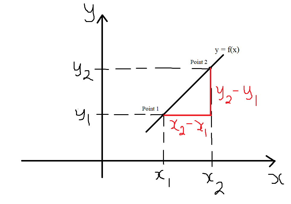
$
Point\;1\;\;(x_1, y_1) \\[3ex]
x_1 = initial\;\;value\;\;of\;\;x \\[3ex]
y_1 = initial\;\;value\;\;of\;\;y \\[3ex]
Point\;2\;\;(x_2, y_2) \\[3ex]
x_2 = final\;\;value\;\;of\;\;x \\[3ex]
y_2 = final\;\;value\;\;of\;\;y \\[3ex]
Change = final\;\;value - initial\;\;value \\[3ex]
Change\;\;in\;\;x = \Delta x = x_2 - x_1 \\[3ex]
Change\;\;in\;\;y = \Delta y = y_2 - y_1 \\[3ex]
Slope,\;\;m \\[3ex]
= \dfrac{\Delta y}{\Delta x} \\[5ex]
= \dfrac{y_2 - y_1}{x_2 - x_1} \\[5ex]
$
In this example, both changes are positive.
Hence, the slope is also positive.
As the value of $x$ increases, the value of $y$ also increases.
This implies that the rate of change of $y$ per unit change of $x$ is positive.
Algebra: (Difference Quotient):
(2.) We defined these terms:
(a.) The secant line to a curve is the line segment that intersects two points on the curve.
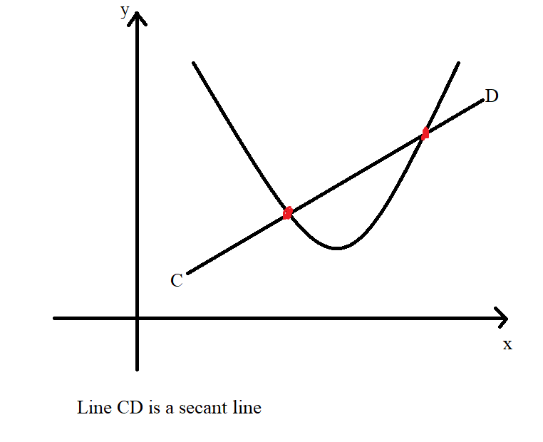
(b.) The tangent line to a curve is the line that touches only one point on the curve.
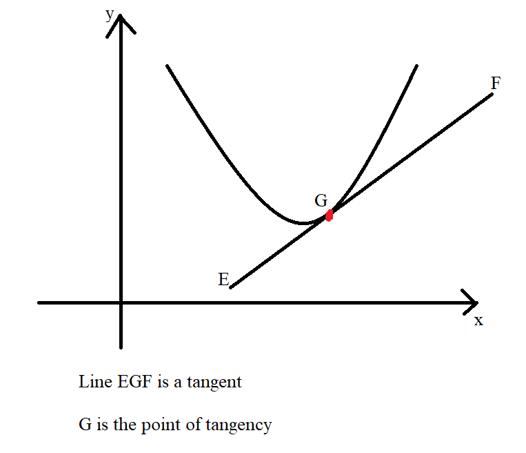
(Notice the terms: intersects, two points, touches, one point)
(3.) We reviewed the Difference Quotient of a function and noted these definitions.
We noted that:
(a.) The difference quotient of a function is the slope of the secant line.
(b.) The derivative of a function is the slope of the tangent line.
(4.) We also noted that for:
the graph of all linear functions (straight-line graph):
the slope of the line is the same at every point on the graph/line.
Depending on the graph, the slope can be positive, negative, zero, or undefined.
Calculus:
But, how do we find the slope of non-linear graphs (curves)?
For example, how do we find the slope of a: parabola? graph of a cubic function? graph of a quartic function? etc.
Well, here comes Calculus!
Because a non-linear graph is not a straight line, the slope is not the same at every point on the graph/curve.
The slope changes/varies (rises, falls, is constant) from one point to another on the graph depending on the intervals at which
the graph is increasing, decreasing, or is constant.
In this case, the slope of the curve is not the same for every point on the curve.
Let us look at the case of a parabola (the graph of a quadratic function).
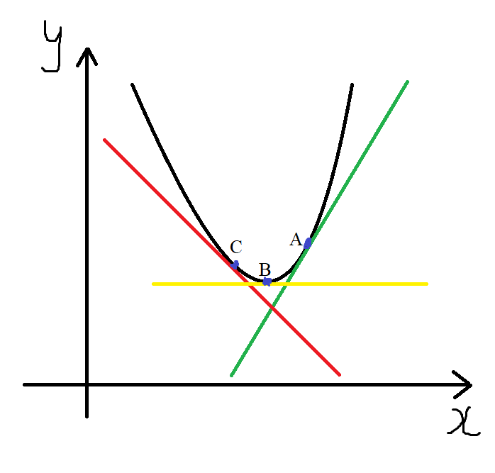
The slope of the three points on the curve are different because the graph is not a straight line. It is a curve.
The slope of point C on the graph is negative because the graph is decreasing at certain intervals in which point C is located (red color)
The slope of point B is zero because the graph is constant at the interval that has point B (yellow color)
The slope of point A is positive because the graps is increasing at some intervals that has point A (green color)
Notice that there are three tangent lines to that curve because each line touches the curve at only one point: Point A or Point B or Point C
The points (Points A, B, and C) are known as points of tangency
The point of tangency is the point of intersection of the tangent line and the curve.
So, the question is: how can we find the slope of any point say point A on a curve?
Finding the Slope of a Curve at a Point of Tangency
(1.) First Approach: Visual Approximation: One way to do this is to approximate it.
This approach involves taking some measurements of the input ($x$) and the output ($y$) value that contains the point of
tangency.
With this approach, it is important to note the scale of the graph on both axis: the $y-axis$ (horizontal axis) and the
$x-axis$ (vertical axis)
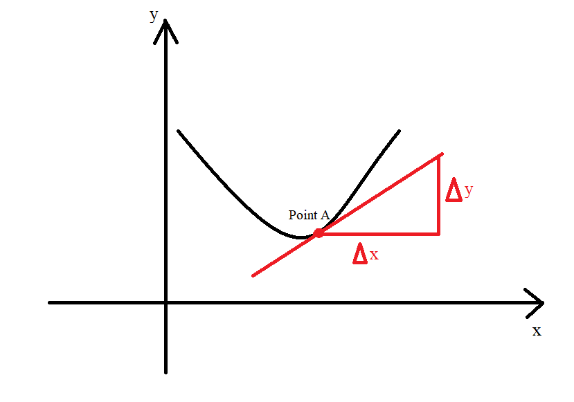
$
Slope\;\;of\;\;the\;\;Curve\;\;at\;\;Point\;A \\[3ex]
m = \dfrac{\Delta y}{\Delta x} \\[5ex]
$
(2.) Second Approach: Difference Quotient
This approach uses a secant line.
It is a more precise approach of approximating the slope of a curve at the point of tangency.
For a secant line, two points are needed.
The first point is the point of tangency.
The second point is another point on the curve.
Remember that we want to find the slope of the curve at Point A
Point A becomes out first point: Point 1
We find another point on the curve and call it Point 2
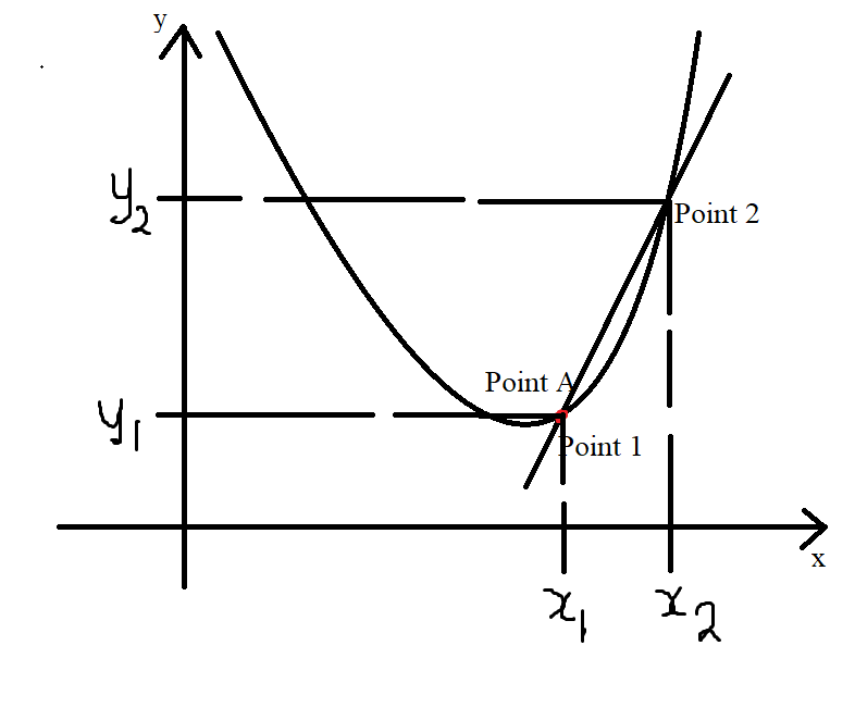
$
Slope\;\;of\;\;the\;\;Curve\;\;at\;\;Point\;A \\[3ex]
Point\;A = Point\;1 = (x_1, y_1) \\[3ex]
Point\;2 = (x_2, y_2) \\[3ex]
y = f(x) \\[3ex]
\Delta x = x_2 - x_1 \\[3ex]
x_2 - x_1 = \Delta x \\[3ex]
x_2 = \Delta x + x_1 \\[3ex]
x_2 = x_1 + \Delta x \\[5ex]
Let:\;\; x_1 = x \\[3ex]
\implies \\[3ex]
y_1 = f(x) \\[3ex]
x_2 = x + \Delta x \\[3ex]
y_2 = f(x_2) \\[3ex]
y_2 = f(x + \Delta x) \\[3ex]
Slope,\;\;m \\[3ex]
= \dfrac{\Delta y}{\Delta x} \\[5ex]
= \dfrac{y_2 - y_1}{x_2 - x_1} \\[5ex]
= \dfrac{f(x + \Delta x) - f(x)}{(x + \Delta x) - x} \\[5ex]
= \dfrac{f(x + \Delta x) - f(x)}{x + \Delta x - x} \\[5ex]
= \dfrac{f(x + \Delta x) - f(x)}{\Delta x} \\[5ex]
Difference\;\;Quotient = DQ \\[3ex]
DQ = \dfrac{f(x + \Delta x) - f(x)}{\Delta x} \\[5ex]
$
This is the Slope of the secant line
It is the average rate of the function at point A (point of tangency)
It is also known as the Difference Quotient because it is a quotient of two differences.
The numerator is a difference.
The simplified denominator was a difference.
Here is the interesting thing:
The second point we chose is a bit distant.
We can choose a point very close to the first point (the point of tangency)
By choosing points closer and closer to the point of tangency (the first point), more accurate approximations of the slope of
the tangent line is obtained.
This implies that as the secant line approaches the tangent line, more accurate approximations of the slope is obtained.
This implies that as the change in $x$: $\Delta x$ approaches zero, more accurate approximations of the slope is obtained.
Hence, the definition of limit is introduced.
(3.) Third Approach: Derivative
This approach uses the limit of the difference quotient as the change in the independent variable approaches zero.
It gives the exact value of the slope of the curve at the point of tangency.
$
\displaystyle{\lim_{\Delta x \to 0}} DQ \\[5ex]
= \displaystyle{\lim_{\Delta x \to 0}} \dfrac{f(x + \Delta x) - f(x)}{\Delta x} \\[5ex]
= \dfrac{dy}{dx} \\[5ex]
\therefore \dfrac{dy}{dx} = \displaystyle{\lim_{\Delta x \to 0}} \dfrac{f(x + \Delta x) - f(x)}{\Delta x} \\[5ex]
\dfrac{dy}{dx} = f'(x) \\[3ex]
So: \\[3ex]
f'(x) = \displaystyle{\lim_{\Delta x \to 0}} \dfrac{f(x + \Delta x) - f(x)}{\Delta x} \\[5ex]
$
This is the Slope of the tangent line
It is the instantaneous rate of the function at Point A (the point of tangency)
It is also known as the Derivative
This gives us the exact value of the slope of the tangent line to the curve at Point A (the point of tangency)
It is the slope of the graph at $(x, f(x))$
Everything must not be $x$
We can use any variable as the independent variable.
Assume we decide to use the variable: $a$ rather than $x$, we have:
$
DQ = \dfrac{f(a + \Delta a) - f(a)}{\Delta a} \\[5ex]
f'(a) = \displaystyle{\lim_{\Delta a \to 0}} \dfrac{f(a + \Delta a) - f(a)}{\Delta a} \\[5ex]
$
The difference quotient is the approximate slope of the graph at $(a, f(a))$
The derivative is the exact slope of the graph at $(a, f(a))$
Newton's Method
also known as the Newton-Raphson Method
Vocabulary Words
numerical analysis, function, zeros, roots, Newton's method, Newton-Raphson Method, initial guess,
initial approximation, iteration, absolute difference,
Numerical Analysis is the branch of mathematics that uses numerical methods/computations to determine
approximate solutions to mathematical problems.
One of the numerical methods is the Newton's method.
Newton's Method is the numerical method used to determine the approximate roots of functions.
For some functions, it is very challenging to determine the zeros algebraically
The roots of those kinds of functions are determined graphically and/or technologically using
several applications such as the Wolfram|Alpha and the applicable TI-84 family graphing calculators among others.
Alternatively, we can determine the roots of those functions using numerical methods
One of those numerical methods is the Newton's method.
Using Newton's Method:
Assume $x$ is a solution (zero) of the function: $f(x)$ and $f(x)$ is differentiable on an open interval containing $x$
To determine the approximate value of $x$:
(1.) Make an initial approximation (guess) for a value say $x_1$ that is close to $x$
Sometimes, you may be given the initial guess.
However, if you are not given the initial guess, use a graphing utility or an applicable calculator to determine the
actual zero, and then make an initial guess close to that value.
(2.) Determine a new approximation, say $x_2$ and subsequent approximations using the formula:
$
x_{n + 1} = x_n - \dfrac{f(x)}{f'(x)} \\[5ex]
$
(3.) Keep determining new approximations until the absolute value of the difference (absolute difference) between
an approximation, $x_n$ and the subsequent approximation, $x_{n + 1}$ is within a desired accuracy say $0.000001$
In other words, keep getting $x_n$ and $x_{n + 1}$ until $|x_n - x_{n + 1}|$ is zero or very close to zero
So, after the initial guess, $x_1$, find $x_2$ and determine the difference
If $|x_1 - x_2|$ is not close to zero, find $x_3$ using the formula in (2.)
Then, find the absolute difference between $x_2$ and $x_3$: $|x_2 - x_3|$
Keep repeating the process until the absolute difference is zero or very close to zero.
Each successive application (repetition) of using an approximation to determine the next approximation is known as
an iteration
So, in other words; you keep iterating until the absolute difference is zero or very close to zero.
The final approximation (the value of $x_{n + 1}$ whose absolute difference with $x_n$ gave zero) then becomes the
zero of the function.
Let us solve some examples.
Let us begin with an example that can be solved algebraically.
Example 1: The equation:
$x^2 = -12x - 20$
[Question (25.) on the Quadratic Equations website] can be solved algebraically:
(By Factoring, Completing the Square, and Quadratic Formula)
It can also be solved graphically.
Based on the solutions in that example, one of the roots of the equation is $2$
Transform the equation to a function and using an initial guess of $x = -1$, determine at least one zero of the function by
performing iterations of Newton's method until the difference between two successive approximations when rounded to
three decimal places is within 0.001
Solution 1:
$
x^2 = -12x - 20 \\[3ex]
x^2 + 12x + 20 = 0 \\[3ex]
x^2 + 12x + 20 = f(x) \\[3ex]
f(x) = x^2 + 12x + 20 \\[3ex]
f'(x) = 2x + 12 \\[3ex]
x_{n + 1} = x_n - \dfrac{f(x)}{f'(x)} \\[5ex]
\implies \\[3ex]
x_{n + 1} = x_n - \dfrac{x_n^2 + 12x_n + 20}{2x_n^2 + 12}
$
| $n$ | $1$ | $2$ | $3$ |
| $x_n$ | $-1$ | $-1.9$ | $-1.998780488$ |
| $x_n^2$ | $1$ | $3.61$ | $3.995123438$ |
| $12x_n^2$ | $-12$ | $-22.8$ | $-23.98536586$ |
| $20$ | $20$ | $20$ | $20$ |
| $\color{purple}{x_n^2 + 12x_n + 20}$ | $9$ | $0.81$ | $0.009757578$ |
| $2x_n$ | $-2$ | $-3.8$ | $-3.997560976$ |
| $12$ | $12$ | $12$ | $12$ |
| $\color{purple}{2x_n + 12}$ | $10$ | $8.2$ | $8.002439024$ |
| $\color{purple}{\dfrac{x_n^2 + 12x_n + 20}{2x_n + 12}}$ | $0.9$ | $0.0987804878$ | $0.0012193255$ |
| $\color{red}{x_n - \dfrac{x_n^2 + 12x_n + 20}{2x_n + 12}}$ | $-1.9$ | $-1.998780488$ | $\color{red}{-1.999999814}$ |
$
\underline{Iteration\;2} \\[3ex]
|x_n - x_{n + 1}| \\[3ex]
= |-1.9 - (-1.998780488)| \\[3ex]
= |-1.9 + 1.998780488| \\[3ex]
= |0.098780488| \\[3ex]
= 0.098780488 \\[3ex]
\approx 0.099 \\[3ex]
0.099 \gt 0.001 ...CONTINUE \\[3ex]
\underline{Iteration\;3} \\[3ex]
|x_n - x_{n + 1}| \\[3ex]
= |-1.998780488 - (-1.999999814)| \\[3ex]
= |-1.998780488 + 1.999999814| \\[3ex]
= |0.001219326| \\[3ex]
= 0.001219326 \\[3ex]
\approx 0.001 ... STOP \\[3ex]
\therefore at\;\;least\;\;one\;\;zero\;\;of\;\;x^2 = -12x - 20 \\[3ex]
= x_{n + 1} \\[3ex]
= x_n - \dfrac{x_n^2 + 12x_n + 20}{2x_n^2 + 12} \\[5ex]
= -1.999999814 \\[3ex]
\approx -2 \\[3ex]
$
Student: Mr. C, must we always use a table?
Teacher: The use of a table is optional.
I used it in order to simplify the method.
You must not use a table.
You can substitute the values directly in the method.
Let us solve more examples where we do not need tables.
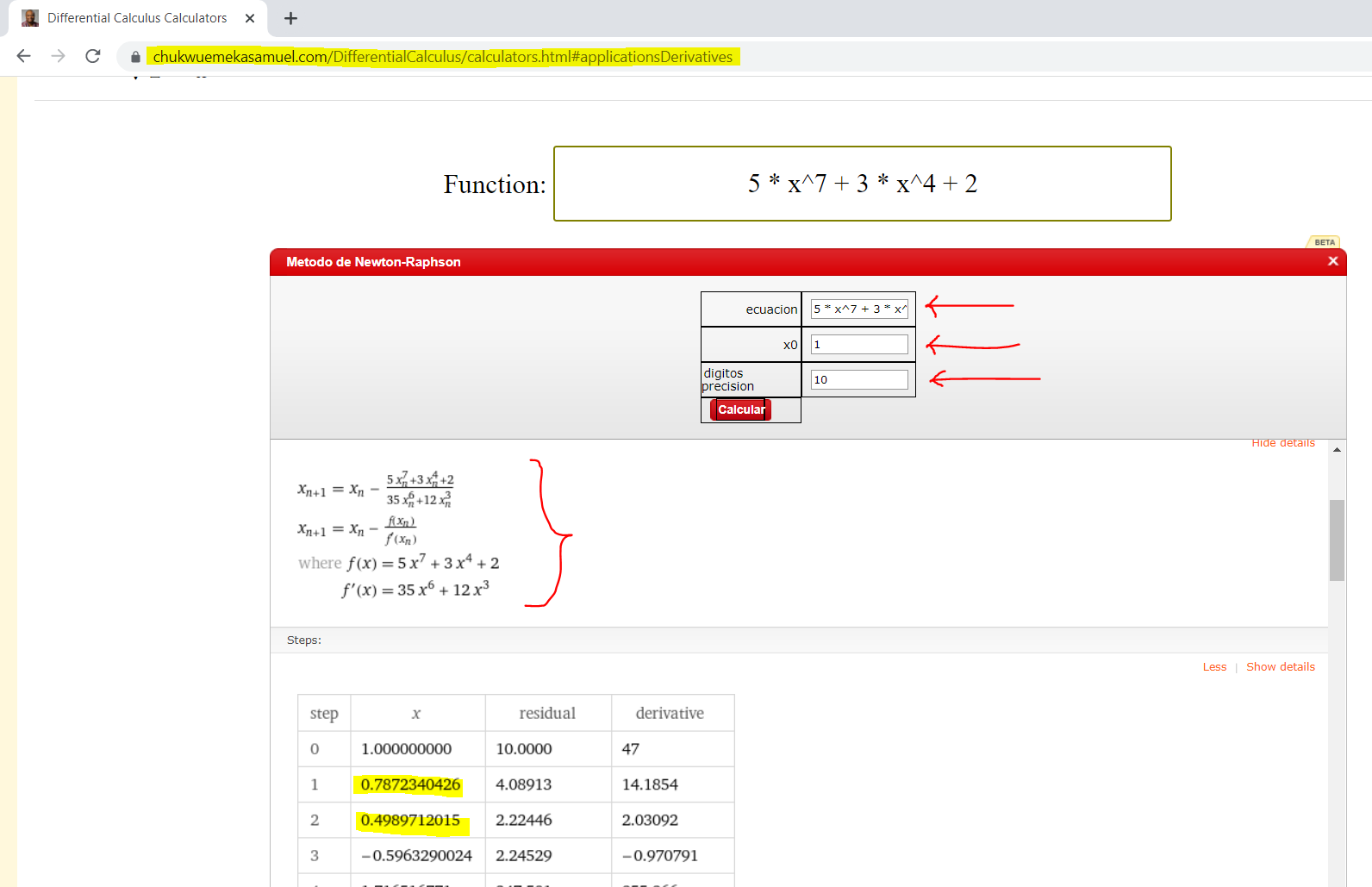
Example 2: Use Newton's method to approximate a root of the equation: $5x^7 + 3x^4 + 2 = 0$ as follows.
Let $x_1 = 1$ be the initial approximation.
Determine the second, $x_2$ and third, $x_3$ approximations.
Carry at least 4 decimal places through your calculations.
Solution 2
$
5x^7 + 3x^4 + 2 = 0 \\[3ex]
5x^7 + 3x^4 + 2 = f(x) \\[3ex]
f(x) = 5x^7 + 3x^4 + 2 \\[3ex]
f'(x) = 35x^6 + 12x^3 \\[3ex]
x_{n + 1} = x_n - \dfrac{f(x)}{f'(x)} \\[5ex]
\implies \\[3ex]
x_{n + 1} = x_n - \dfrac{5x_n^7 + 3x_n^4 + 2}{35x_n^6 + 12x_n^3} \\[5ex]
x_1 = 1 \\[3ex]
x_2 = x_1 - \dfrac{5 * x_1^7 + 3 * x_1^4 + 2}{35 * x_1^6 + 12 * x_1^3} \\[5ex]
= 1 - \dfrac{5(1)^7 + 3(1)^4 + 2}{35(1)^6 + 12(1)^3} \\[5ex]
= 1 - \dfrac{5(1) + 3(1) + 2}{35(1) + 12(1)} \\[5ex]
= 1 - \dfrac{5 + 3 + 2}{35 + 12} \\[5ex]
= 1 - \dfrac{10}{47} \\[5ex]
= 1 - 0.2127659574 \\[3ex]
= 0.7872340426 \\[5ex]
x_3 = x_2 - \dfrac{5 * x_2^7 + 3 * x_2^4 + 2}{35 * x_2^6 + 12 * x_2^3} \\[5ex]
= 0.7872340426 - \dfrac{5(0.7872340426)^7 + 3(0.7872340426)^4 + 2}{35(0.7872340426)^6 + 12(0.7872340426)^3} \\[5ex]
$
Student: Why don't we round the value of $x_2$?
The calculations involves a lot of values...too much
Besides, the question says we should carry at least 4 decimal places through the calculations.
Teacher: Nice observation.
We can round the value of $x_2$ and the intermediate values in the calculations to 4 decimal place.
However, it is better that we use the exact values and compute it with the TI-84 Plus calculator
Let's do it.
Step 1:
Enter the function (the function at the numerator)
This is the $Y_1$
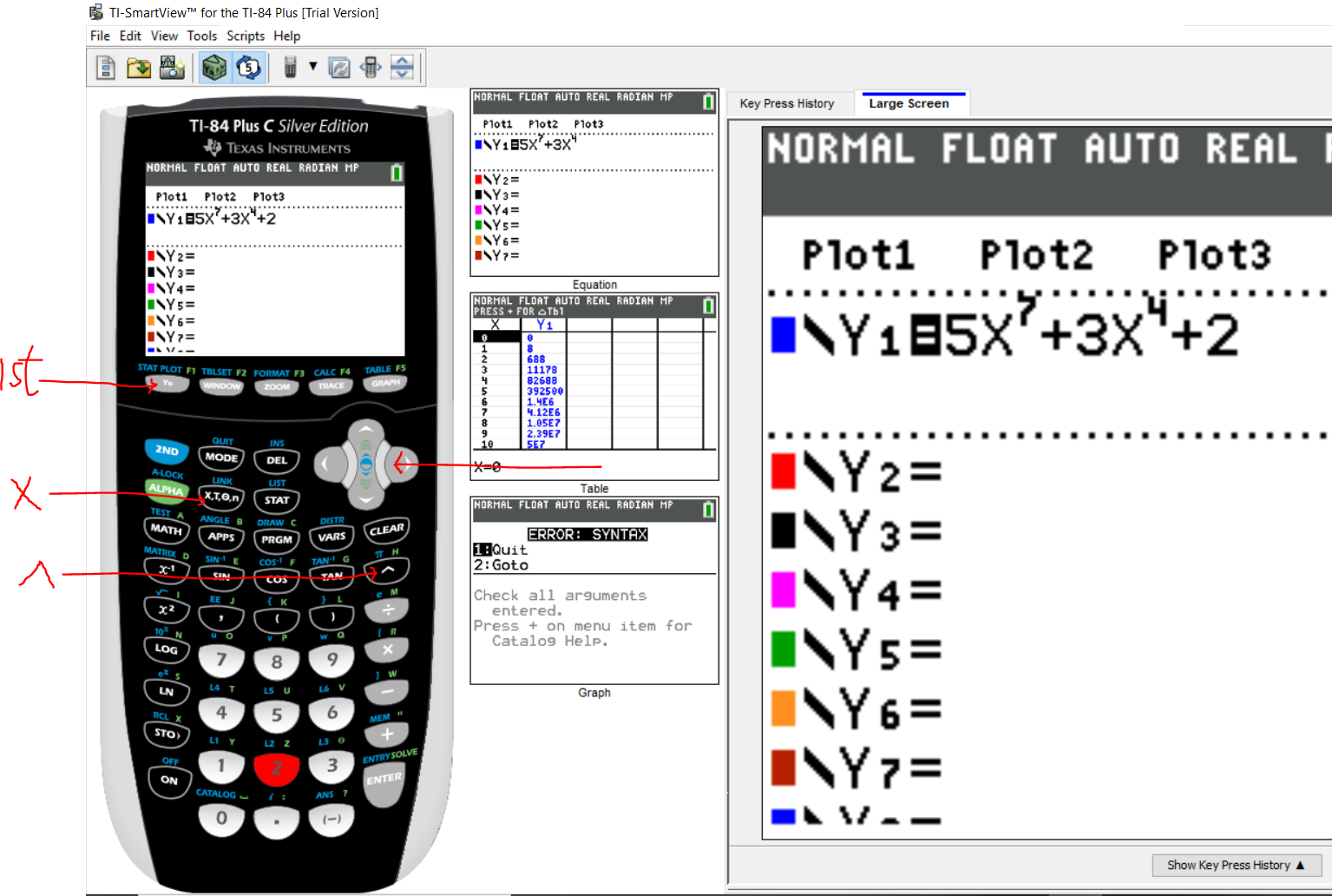
Press the ENTER key to enter the derivative (the function at the denominator)
This is the $Y_2$
Step 2:

Press the ENTER key
Press the 2ND function key
Press the MODE key (to QUIT)
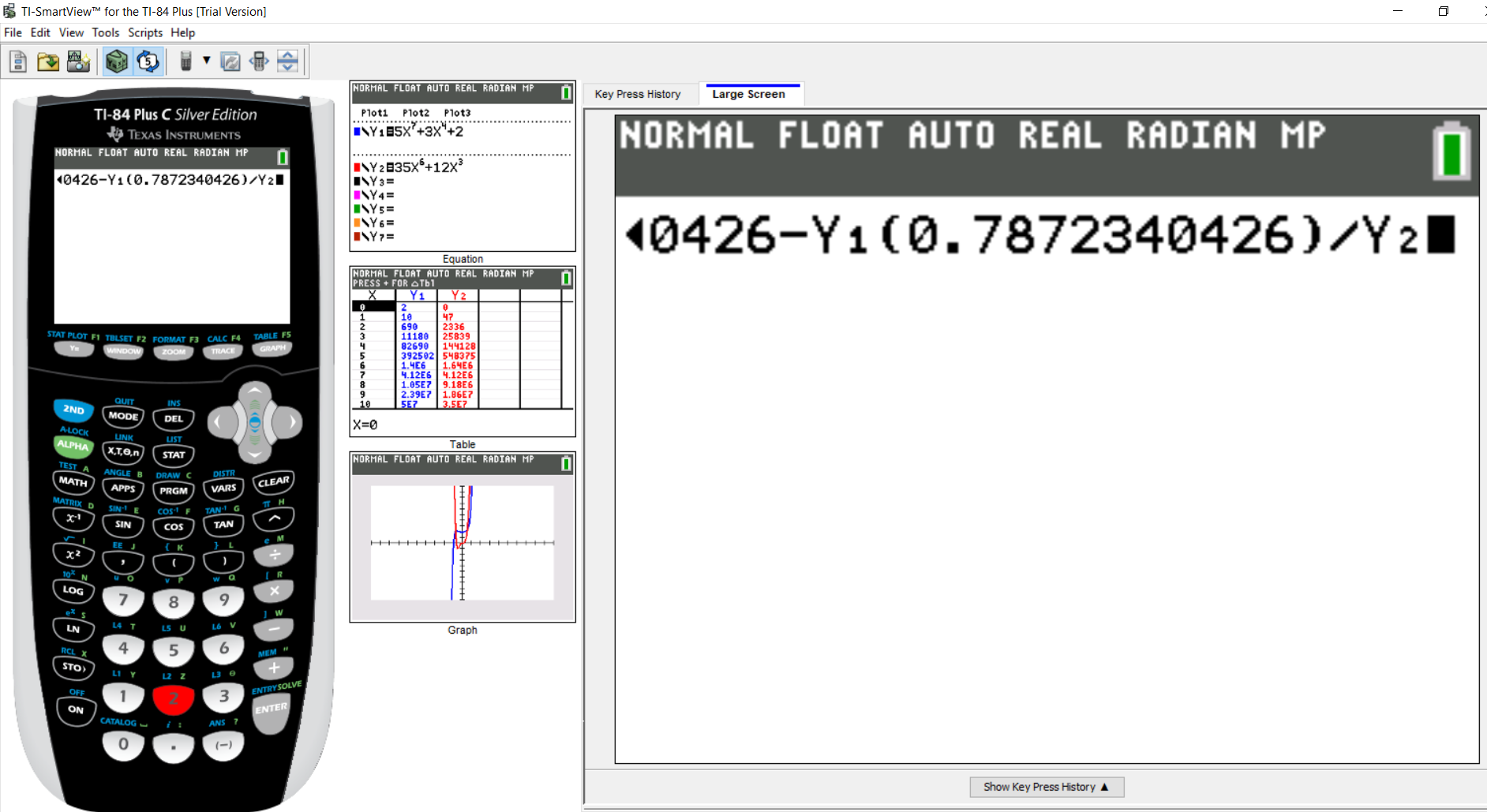
Step 3: Part 1:
Let us enter the Newton's method to calculate $x_3$
Enter the first value (the expression on the left...the value of $x_2$)
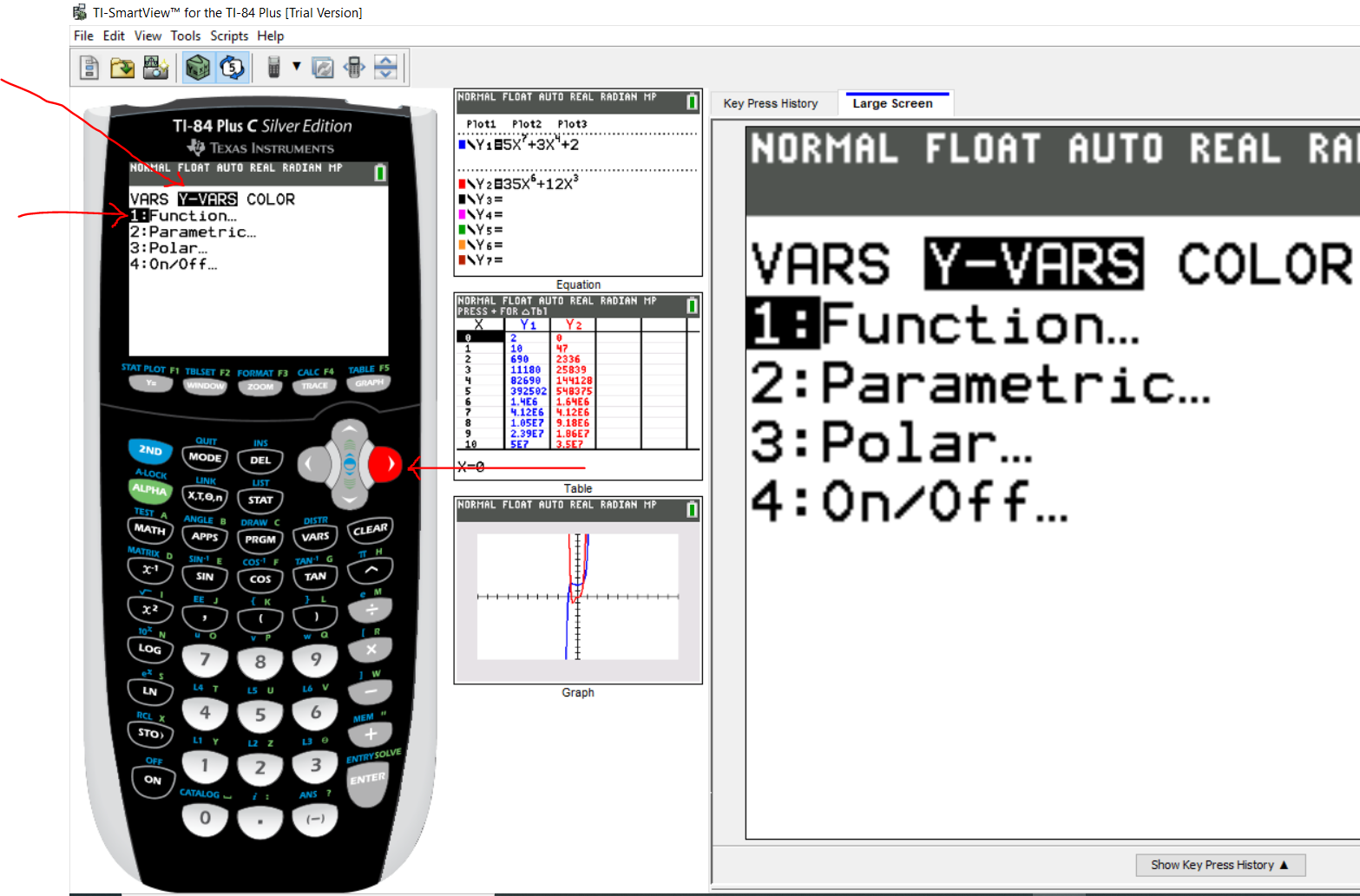
Step 3: Part 2:
Press the VARS (variables) key
Use the right cursor/arrow to move to Y-VARS (y-variables) menu
By default, it is positioned on 1: Function...
Step 3: Part 3:
Press the ENTER key or the number 1 key (it does not matter)
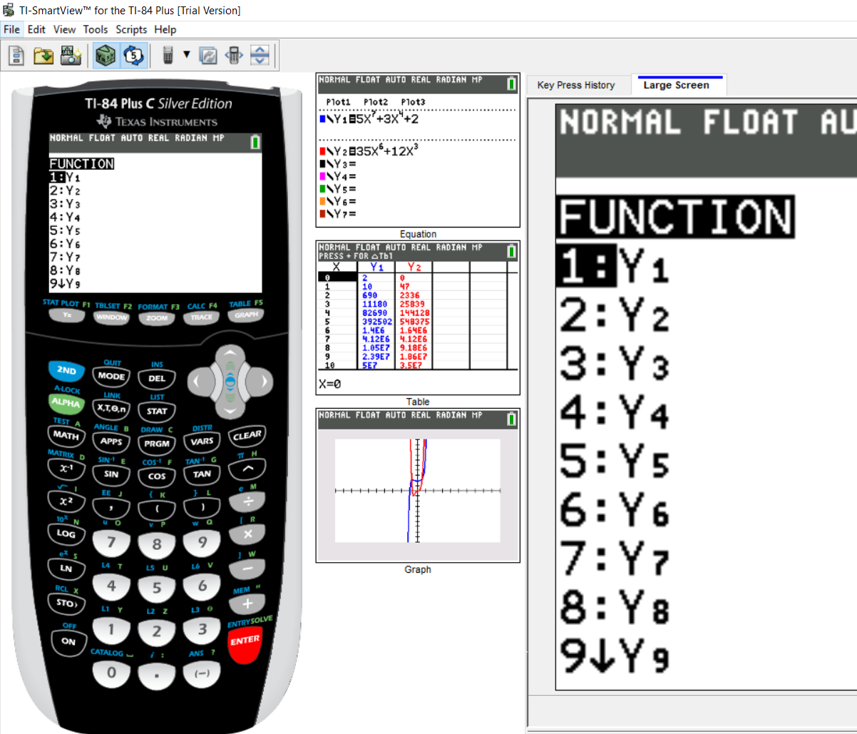
Step 3: Part 4:
By default, it is positioned at $1:Y_1$
The numerator is the $Y_1$
So, press the ENTER key or the number 1 key (it does not matter)
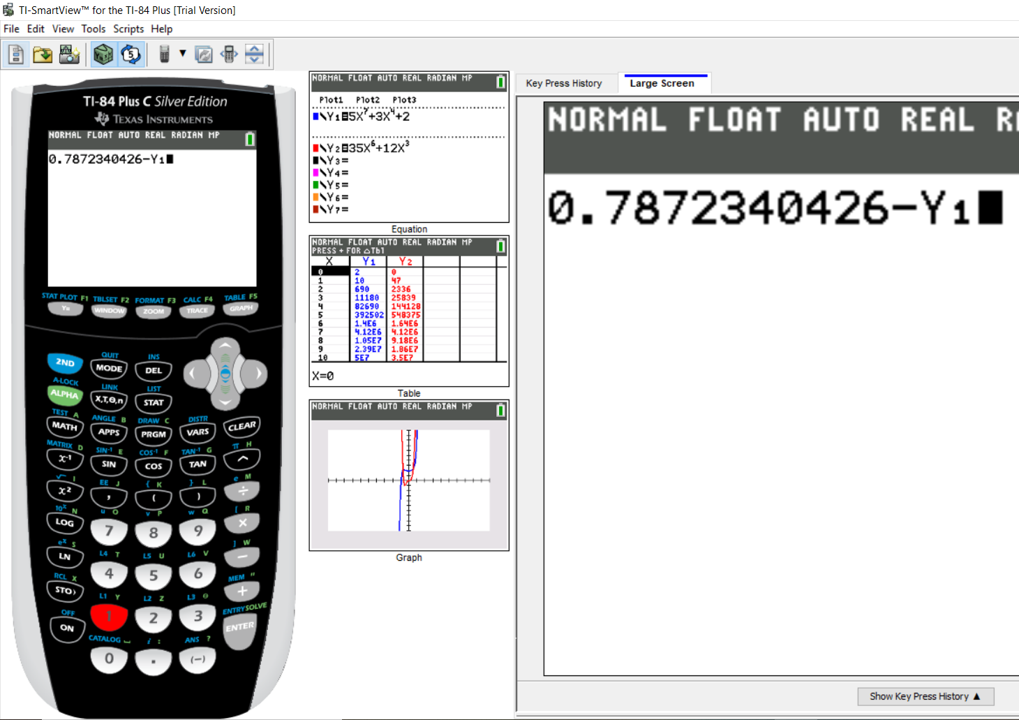
Step 3: Part 5:
Put the value of $x_2$ as the argument
In other words, put a parenthesis and type the value of $x_2$
Then, press the division symbol
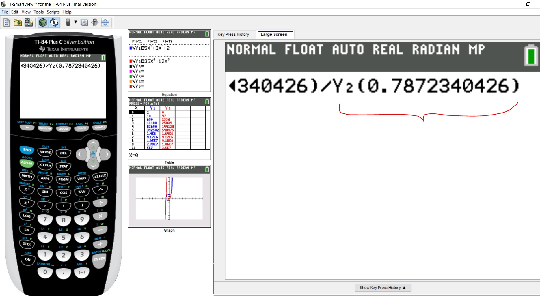
Step 3: Part 6:
Let us repeat the same process for the denominator, $Y_2$
So, press the VARS key and move the right arrow to Y-VARS
Press the Number 1 or press the ENTER key
Then, in the next window, because we need to use the denominator; we shall press Number 2
Alternatively, we can use the down arrow/cursor to move to $2: Y_2$ and press the ENTER key
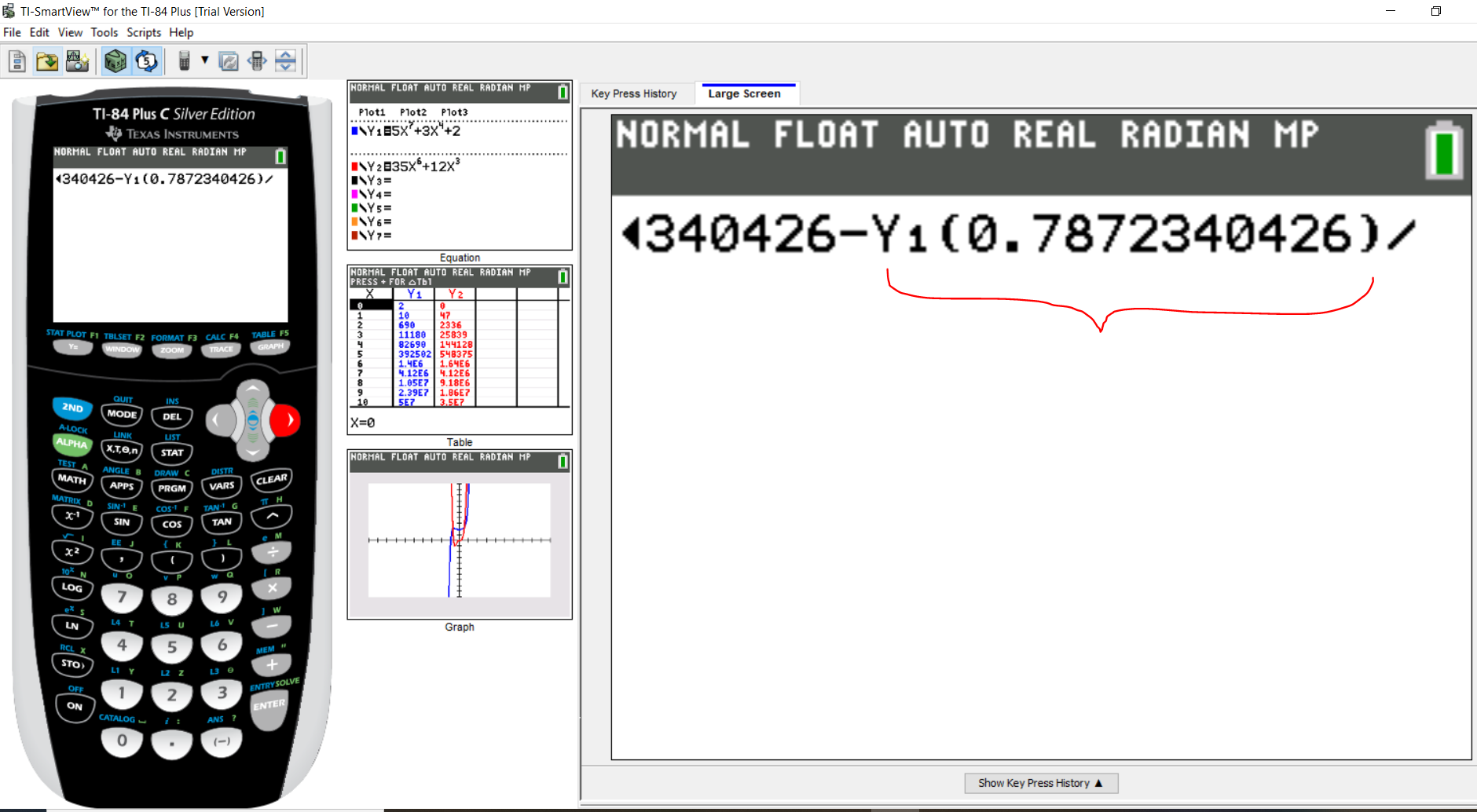
Step 3: Part 7:
Enter the argument for $Y_2$ (same value as $x_2$)
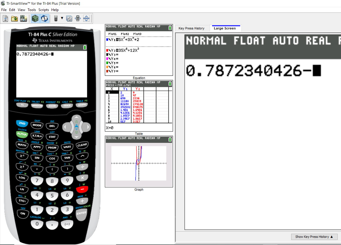
Step 4:
Press the ENTER key to do the calculation
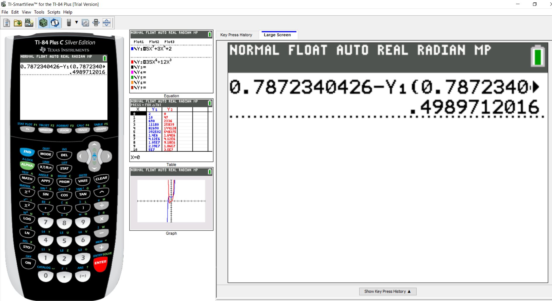
$
x_3 = 0.4989712015 \\[3ex]
$
Going forward, we shall use the TI-84 Plus Family calculator (or other approved applicable calculator).
Any calculator in that family series of TI-84 should perform this kind of calculation.
For homework assignments, you may verify your answers with the
Wolfram|Alpha widget calculator
Convergence and Non-convergence of Newton's Method
As seen in the first example, we were able to determine the approximate zero of the function (the final approximation).
The second method is also applicable...if we kept iterating with the formula
In those two cases, we determined the convergence of the Newton's method.
In other words, the Newton's method is said to converge if the approximate zero of the function can be determined.
For some other cases, the Newton's method may not converge.
What are those cases?
Conditions for the Non-convergence of Newton's Method
The conditions where Newton's method may not converge are:
(1.) The derivative of an approximation, say $x_n$ is zero for some value of $n$
In other words, if $f'(x_n) = 0$ for some $n$
(2.) The limit to infinity of an approximation, say $x_n$ does not exist.
In other words, if $\displaystyle{\lim_{n \rightarrow \infty}}\: x_n$ does not exist (DNE)
In this case, Newton's method only converges at the exact value of the zero. It does not converge at any other value
besides the exact value of the zero of the function.
Optimization
Vocabulary Words
minimum, minima, maximum, maxima, extremum, extrema, optimum, optima, optimization,
Minimum Distance (Point on Curve to Point on Graph)
Calculus (Derivatives) is also used to:
(1.) determine a point (or points) on a curve (on a graph) at a minimum distance from a point on the graph.
(2.) determine the minimum distance between the two points.
Student: I thought we can just use the Distance Formula to determine the distance between two points.
Why use Derivatives?
Teacher: We shall use both the Distance Formula and Derivatives
Student: I do not understand why we need to use Calculus
Teacher: Calculus makes it much easier for us to find the exact point, rather than testing several points
No worries, it will make more sense when we solve some examples.
Given: a curve on a graph, equation of the curve, a point on the graph (not on the curve)
To Determine: a point or points on the curve closest to the point on the graph
So, we are given a point that is on the graph but not on the curve
We are asked to find a point (or points as the case may be) on the curve that is closest to the point on the graph.
In other words, we want to determine a point (points) on the curve whose distance from the point on the graph is
a minimum.
Assume $y = f(x)$
The steps are:
(1.) Express y in terms of x
In other words, isolate y
(2.) Define the two points: the given point and the point to be determined
The first point is the given point.
The second point is the point to be determined.
Note the co-ordinates of each point.
For the y-coordinate of the second point, substitute for the value of y that was isolated in (1.)
(3.) Apply the Distance Formula for the two points.
Simplify the radicand (expression inside the square root).
(4.) Minimize the distance between the two points by minimizing the radicand.
Let the simplified radicand in the Distance Formula be a function of x
As the radicand is minimized, the square root of the radicand is minimized, and hence the distance
(using the Distance Formula) is minimized.
Why is it important that we minimize the distance?
Remember, we are looking for a point on the curve on the curve that is closest to the given point.
Hence, it is important that we minimize the distance so we can get the closest point.
So, we do not need to work with the entire square root (distance formula). Once we minimize the radicand, the entire
square root/distance formula is also minimized.
(a.) Determine the critical values of the radicand.
(b.) Write the intervals based on the criitcal values.
(c.) Test specific values within each interval.
(d.) Examine the behavior within each interval.
(e.) Apply the First Derivative Test to determine the critical value(s) that yields a relative minimum
(for an actual graph of a function).
The critical value(s) that would yield a relative minimum for an actual graph are the value(s) on the curve whose distance
is closest to the point on the graph.
Example 3: For the parabola: $x^2 - 2x - 4y = 8$
(a.) Determine the point(s) on the curve closest to the point (1, 6)
(b.) Use a graph to verify that your solution is reasonable.
Solution 3:
Let the point on the curve closest to the point (1, 6) be $x_2, y_2$
$
\underline{First\;\;Step:\;\;Isolate\;\;y} \\[3ex]
x^2 - 2x - 4y = 8 \\[3ex]
x^2 - 2x - 8 = 4y \\[3ex]
4y = x^2 - 2x - 8 \\[3ex]
y = \dfrac{x^2 - 2x - 8}{4} \\[5ex]
y = \dfrac{x^2}{4} - \dfrac{2x}{4} - \dfrac{8}{4} \\[5ex]
y = \dfrac{x^2}{4} - \dfrac{x}{2} - 2 \\[5ex]
\underline{Second\;\;Step:\;\;Define\;\;Points} \\[3ex]
1st\;\;Point = (1, 6) \\[3ex]
x_1 = 1 \\[3ex]
y_1 = 6 \\[3ex]
2nd\;\;Point = (x_2, y_2)\\[3ex]
x_2 = x \\[3ex]
y_2 = y = \dfrac{x^2}{4} - \dfrac{x}{2} - 2 \\[5ex]
\underline{Third\;\;Step:\;\;Distance\;\;Formula} \\[3ex]
distance = \sqrt{(x_2 - x_1)^2 + (y_2 - y_1)^2} \\[3ex]
= \sqrt{(x - 1)^2 + (y - 6)^2} \\[3ex]
Substitute\;\;for\;\;x_2\;\;and\;\;y_2 \\[3ex]
= \sqrt{(x - 1)^2 + (y - 6)^2} \\[3ex]
Substitute\;\;for\;\;y \\[3ex]
= \sqrt{(x - 1)^2 + \left(\dfrac{x^2}{4} - \dfrac{x}{2} - 2 - 6\right)^2} \\[5ex]
= \sqrt{(x - 1)^2 + \left(\dfrac{x^2}{4} - \dfrac{x}{2} - 8\right)^2} \\[5ex]
= \sqrt{(x - 1)(x - 1) + \left(\dfrac{x^2}{4} - \dfrac{x}{2} - 8\right)\left(\dfrac{x^2}{4} - \dfrac{x}{2} - 8\right)} \\[5ex]
= \sqrt{(x^2 - x - x + 1) + \left(\dfrac{x^4}{16} - \dfrac{x^3}{8} - \dfrac{8x^2}{4} - \dfrac{x^3}{8} + \dfrac{x^2}{4} + \dfrac{8x}{2} - \dfrac{8x^2}{4} + \dfrac{8x}{2} + 64\right)} \\[5ex]
= \sqrt{(x^2 - 2x + 1) + \left(\dfrac{x^4}{16} - \dfrac{2x^3}{8} - \dfrac{15x^2}{4} + \dfrac{16x}{2} + 64\right)} \\[5ex]
= \sqrt{(x^2 - 2x + 1) + \left(\dfrac{x^4}{16} - \dfrac{x^3}{4} - \dfrac{15x^2}{4} + 8x + 64\right)} \\[5ex]
= \sqrt{x^2 - 2x + 1 + \dfrac{x^4}{16} - \dfrac{x^3}{4} - \dfrac{15x^2}{4} + 8x + 64} \\[5ex]
= \sqrt{\dfrac{x^4}{16} - \dfrac{x^3}{4} + \dfrac{4x^2}{4} - \dfrac{15x^2}{4} - 2x + 8x + 1 + 64} \\[5ex]
= \sqrt{\dfrac{x^4}{16} - \dfrac{x^3}{4} - \dfrac{11x^2}{4} + 6x + 65} \\[5ex]
\underline{Fourth\;\;Step:\;\;Minimize\;\;the\;\;Radicand} \\[3ex]
Radicand = f(x) = \dfrac{x^4}{16} - \dfrac{x^3}{4} - \dfrac{11x^2}{4} + 6x + 65 \\[5ex]
f'(x) = \dfrac{4x^3}{16} - \dfrac{3x^2}{4} - \dfrac{22x}{4} + 6 \\[5ex]
f'(x) = \dfrac{x^3}{4} - \dfrac{3x^2}{4} - \dfrac{11x}{2} + 6 \\[5ex]
f'(x)\;\; is\;\;defined\;\;for\;\;all\;\;values\;\;of\;\;x \\[3ex]
f'(x) = 0 \\[3ex]
\implies \\[3ex]
\dfrac{x^3 - 3x^2 - 22x + 24}{4} = 0 \\[5ex]
x^3 - 3x^2 - 22x + 24 = 0 \\[3ex]
\underline{Determine\;\;the\;\;critical\;\;values} \\[3ex]
Try\;\;x = 1 \\[3ex]
1^3 - 3(1)^2 - 22(1) + 24 = 1 - 3 -22 + 24 = 0 \\[3ex]
x = 1 \;\;is\;\;a\;\;critical\;\;value \\[3ex]
x - 1 \;\;is\;\;a\;\;critical\;\;factor \\[3ex]
Using\;\;Long\;\;Division\;\;to\;\;find\;\;other\;\;factors \\[3ex]
\begin{array}{c|c}
&x^2 - 2x - 24 \hspace{3em} \\
\hline
x - 1 & x^3 - 3x^2 - 22x + 24 \\
&- \hspace{10em} \\
&x^3 - x^2 \hspace{5.5em} \\
\hline
&-2x^2 - 22x \hspace{1em} \\
&- \hspace{8em} \\
&-2x^2 + 2x \hspace{1.5em} \\
\hline
&\hspace{4em} -24x + 24 \\
&- \hspace{2em} \\
&\hspace{4em} -24x + 24 \\
\hline
&\hspace{8em} 0 \\
\end{array} \\[5ex]
Quotient = x^2 - 2x - 24 = 0 \\[3ex]
\implies \\[3ex]
(x + 4)(x - 6) = 0 \\[3ex]
x + 4 = 0 \;\;\;OR\;\;\; x - 6 = 0 \\[3ex]
x = -4 \;\;\;OR\;\;\; x = 6 \\[3ex]
\therefore the\;\;critical\;\;values\;\;are:\;\; x = -4,\;\;\;x = 1,\;\;\; x = 6 \\[3ex]
$
The critical values are represented by Points D, E, F
The intervals are the regions bounded by the inequalities within the test values.
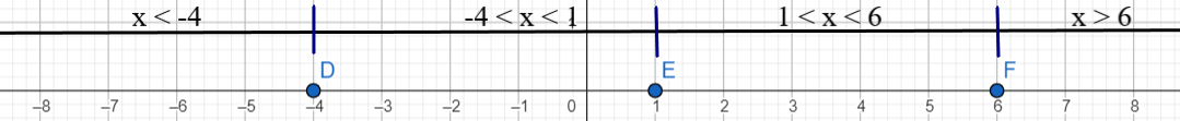
| Intervals | $x \lt 4$ | $-4 \lt x \lt 1$ | $1 \lt x \lt 6$ | $x \gt 6$ |
| Test Values | $x = -8$ | $x = -2$ | $x = 2$ | $x = 8$ |
| $\dfrac{x^3}{4}$ | $-128$ | $-2$ | $2$ | $128$ |
| $-\dfrac{3x^2}{4}$ | $-48$ | $-3$ | $-3$ | $-48$ |
| $-\dfrac{11x}{2}$ | $44$ | $11$ | $-11$ | $-44$ |
| $6$ | $6$ | $6$ | $6$ | $6$ |
| $f'(x)$ | $-126$ | $12$ | $-6$ | $42$ |
| Behavior | Decreasing | Increasing | Decreasing | Increasing |
| For an actual graph of a function |
$x = -4$ yields a relative minimum $x = 1$ yields a relative maximum $x = 6$ yields a relative minimum |
|||
|
For points on a curve closest to a point (1, 6) on the graph (Minimum distance) |
$x = -4$ and $x = 6$ are the values. Let us find the points. |
|||
$
\underline{Points\;\;on\;\;the\;\;curve} \\[3ex]
y = \dfrac{x^2}{4} - \dfrac{x}{2} - 2 \\[5ex]
when\;\; x = -4 \\[3ex]
y = \dfrac{(-4)^2}{4} - \dfrac{-4}{2} - 2 \\[5ex]
= \dfrac{16}{4} - (-2) - 2 \\[5ex]
= 4 + 2 - 2 \\[3ex]
= 4 \\[3ex]
First\;\;Point = (-4, 4) \\[3ex]
when\;\; x = 6 \\[3ex]
y = \dfrac{6^2}{4} - \dfrac{6}{2} - 2 \\[5ex]
= \dfrac{36}{4} - 3 - 2 \\[5ex]
= 9 - 3 - 2 \\[3ex]
= 4 \\[3ex]
Second\;\;Point = (6, 4) \\[3ex]
$
(b.) The graph of the function and the points are shown:
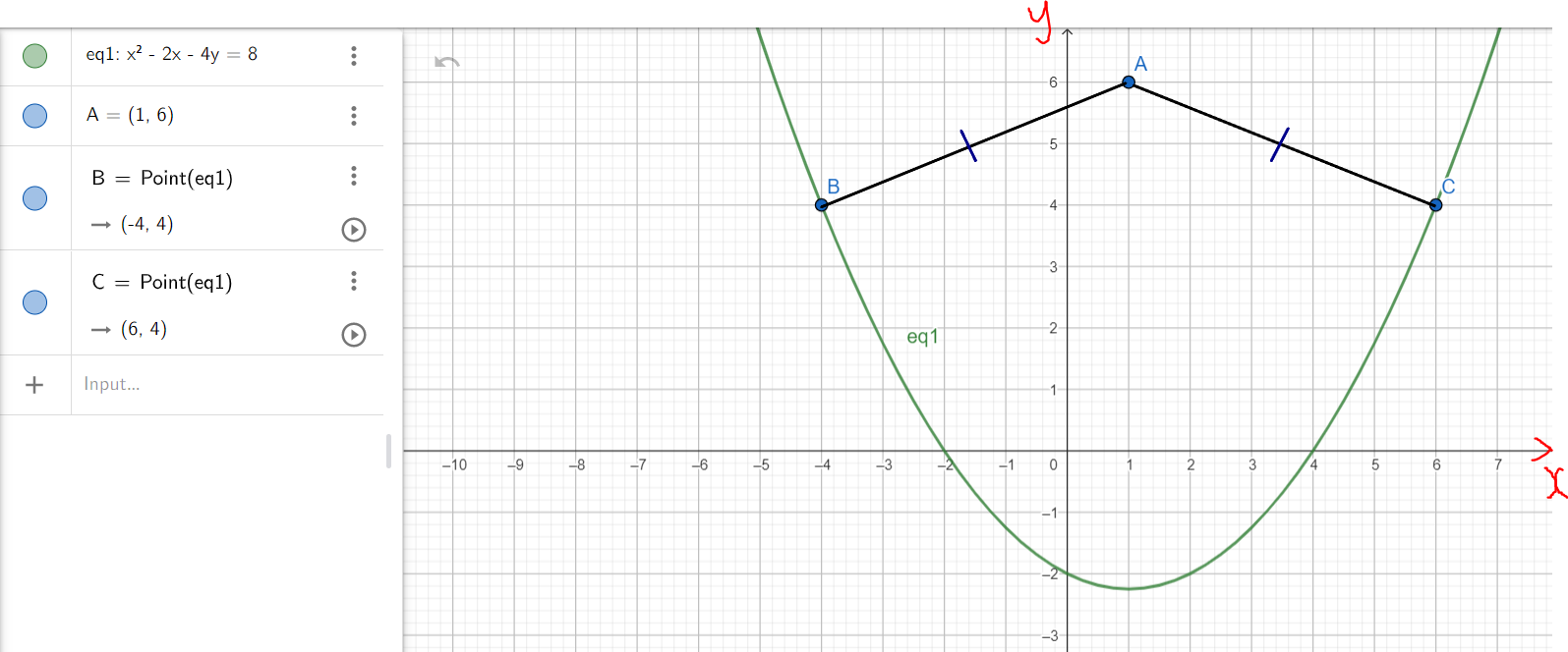
The distance from either point on the curve to the point on the graph is the same.
It is also the minimum distance from any point on the curve to that point (1, 6) on the graph.
$
|AB| = |AC| = minimum\;\;distance \\[3ex]
\underline{Distance\;AB} \\[3ex]
Point\;A = (x_1, y_1) = (1, 6) \\[3ex]
x_1 = 1 \\[3ex]
y_1 = 6 \\[3ex]
Point\;C = (x_2, y_2) = (-4, 4) \\[3ex]
x_2 = -4 \\[3ex]
y_2 = 4 \\[3ex]
|AB| \\[3ex]
= \sqrt{(x_2 - x_1)^2 + (y_2 - y_1)^2} \\[3ex]
= \sqrt{(-4 - 1)^2 + (4 - 6)^2} \\[3ex]
= \sqrt{(-5)^2 + (-2)^2} \\[3ex]
= \sqrt{25 + 4} \\[3ex]
= \sqrt{29}\;\;units \\[3ex]
\underline{Distance\;AC} \\[3ex]
Point\;A = (x_1, y_1) = (1, 6) \\[3ex]
x_1 = 1 \\[3ex]
y_1 = 6 \\[3ex]
Point\;C = (x_2, y_2) = (6, 4) \\[3ex]
x_2 = 6 \\[3ex]
y_2 = 4 \\[3ex]
|AC| \\[3ex]
= \sqrt{(x_2 - x_1)^2 + (y_2 - y_1)^2} \\[3ex]
= \sqrt{(6 - 1)^2 + (4 - 6)^2} \\[3ex]
= \sqrt{5^2 + (-2)^2} \\[3ex]
= \sqrt{25 + 4} \\[3ex]
= \sqrt{29}\;\;units
$
References
Chukwuemeka, S.D (2016, April 30). Samuel Chukwuemeka Tutorials - Math, Science, and Technology. Retrieved from https://www.samuelchukwuemeka.comBerresford, G. C., & Andrew Mansfield Rockett. (2016). Applied Calculus. Cengage Learning.
Calculus. (2016, December 19). Mathematics LibreTexts. https://math.libretexts.org/Bookshelves/Calculus
Larson, R., & Falvo, D. C. (2017). Calculus: An Applied Approach with CalcChat & CalcView. Cengage Learning.
OpenStax | Free Textbooks Online with No Catch. (n.d.). Openstax.org. Retrieved June 10, 2020, from https://openstax.org/subjects/math
Sisson, P., & Szarvas, T. (2016). Single Variable Calculus with Early Transcendentals. Hawkes Learning.
Stroud, K. A., & Booth, D. J. (2001). Engineering Mathematics (5th ed.). Basingstoke: Palgrave.
Tan, S. T. (2004). Applied Calculus for the Managerial, Life, and Social Sciences (5th ed.). Pacific Grove, CA: Brooks/Cole Publishing Company.
Waner, S., & Costenoble, S. (2013). Applied Calculus (6th ed.). Boston, MA: Cengage Learning.
Alpha Widgets Overview Tour Gallery Sign In. (n.d.). Retrieved from http://www.wolframalpha.com/widgets/
Authority (NZQA), (n.d.). Mathematics and Statistics subject resources. www.nzqa.govt.nz. Retrieved December 14, 2020, from https://www.nzqa.govt.nz/ncea/subjects/mathematics/levels/
Desmos. (n.d.). Desmos Graphing Calculator. https://www.desmos.com/calculator
Free Jamb Past Questions And Answer For All Subject 2020. (2020, January 31). Vastlearners. https://www.vastlearners.com/free-jamb-past-questions/
Geogebra. (2019). Graphing Calculator - GeoGebra. Geogebra.org. https://www.geogebra.org/graphing?lang=en
GCSE Exam Past Papers: Revision World. Retrieved April 6, 2020, from https://revisionworld.com/gcse-revision/gcse-exam-past-papers
HSC exam papers | NSW Education Standards. (2019). Nsw.edu.au. https://educationstandards.nsw.edu.au/wps/portal/nesa/11-12/resources/hsc-exam-papers
NSC Examinations. (n.d.). www.education.gov.za. https://www.education.gov.za/Curriculum/NationalSeniorCertificate(NSC)Examinations.aspx
Papua New Guinea: Department of Education. (n.d.). www.education.gov.pg. Retrieved November 24, 2020, from http://www.education.gov.pg/TISER/exams.html
Past Exam Papers | MEHA. (n.d.). Retrieved May 6, 2022, from http://www.education.gov.fj/exam-papers/
School Curriculum and Standards Authority (SCSA): K-12. Past ATAR Course Examinations. Retrieved December 10, 2021, from https://senior-secondary.scsa.wa.edu.au/further-resources/past-atar-course-exams
TI-SmartViewTM Emulator Software for the TI-84 Plus Family - Texas Instruments - US and Canada. (n.d.). Education.ti.com. Retrieved May 6, 2022, from https://education.ti.com/en/software/details/en/ffea90ee7f9b4c24a6ec427622c77d09/sda-ti-smartview-ti-84-plus?msclkid=2fac6524cfb511ecbc87bf63a9cac91b
West African Examinations Council (WAEC). Retrieved May 30, 2020, from https://waeconline.org.ng/e-learning/Mathematics/mathsmain.html